
PRESENTATION:
The MapBiomas Water – Peru initiative (Collection 3) aims to map the dynamics of surface water and glaciers across the national territory from 1985 to 2024.
Unlike MapBiomas Land Cover and Use, the mapping of water bodies in MapBiomas Water is carried out at a monthly scale, and four types of products are available on the platform:
- Monthly and annual maps of water surface.
- Transition maps of water surface between the “Water” and “Non-Water” classes. This product was processed using the annual water surface database;
- Trend maps (increase and decrease) of water surface. This product was calculated using monthly water surface data in 5 km × 5 km grids.
- Maps of types of water bodies, based on their origin.
The glacier mapping is conducted at an annual scale and corresponds to the same dataset displayed in the MapBiomas Land Cover and Use maps. Two types of products are available on the platform:
- Annual maps of glacier cover surface
- Trend maps (increase and decrease) of glacier cover. Similar to the water surface trend data, these were also calculated in 5 km × 5 km grids.
If you wish to consult the complete MapBiomas Water methodology, the ATBD (Algorithm Theoretical Basis Document) is available at this LINK.
If you wish to consult the complete Glacier detection methodology, the ATBD is available at this LINK.
GENERAL METHODOLOGY OF MAPBIOMAS WATER:
- Preprocessing:
The methodology for mapping surface water is based on subpixel classification of Landsat images with less than 70% cloud cover, using the Spectral Mixture Analysis (SMA) algorithm. This algorithm generates endmembers (pure spectral signatures of materials that make up a pixel) from the image bands. The endmembers used are:
- Green vegetation (GV)
- Non-photosynthetic vegetation (NPV)
- Soil
- Clouds
- Shade
- Snow
This subpixel detection approach is useful for characterizing surface water mixed with other components, enabling the mapping of wetlands, floodplains, narrow rivers, and small water bodies.
- Surface Water Detection Algorithm
Once the endmembers for each pixel are obtained, transition rules are applied using a set of linear functions based on fuzzy logic rules. Finally, thresholds are defined for each endmember to determine the degree of certainty that a pixel is classified as water.
Due to the heterogeneity and particularity of Peru’s geography, the classification methodology was adapted for specific regions. In Collection 3, there are 37 subregions covering the entire national territory, and each subregion uses endmembers and thresholds best suited for water detection.
Figure 1 – Stages of surface water classification.
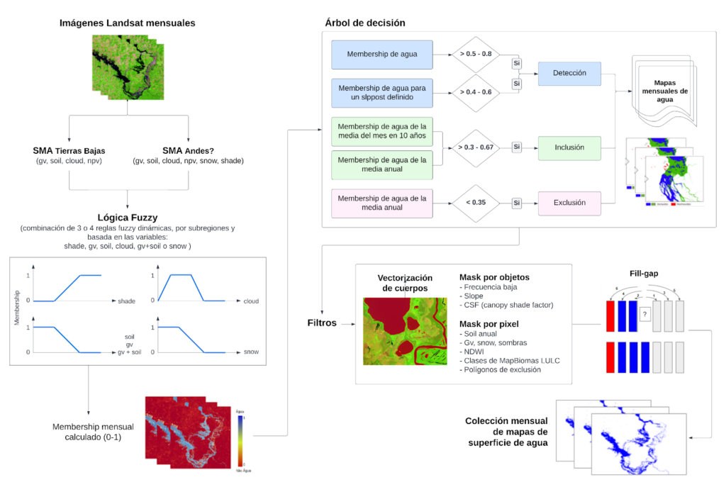
The monthly maps were refined with procedures to restore false negatives and remove false positives, based on auxiliary mosaics (annual and decadal mosaics) and detection thresholds.
Additionally, other false positives were removed considering factors such as slope, frequency, NDWI, CSF, and MapBiomas Land Cover and Use layers. To restore remaining false negatives, an inclusion filter based on a 4-year temporal window was applied.
Finally, monthly surface water maps were generated, from which annual maps (frequency ≥ 6 months) were derived. These in turn serve as inputs for the classification of types of water bodies.
- Types of Water Bodies
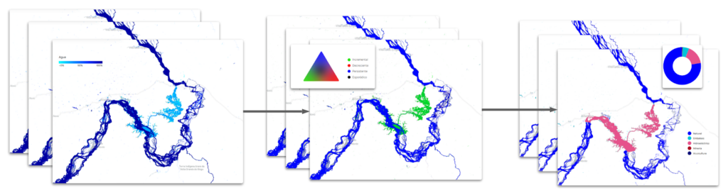
For the classification of water bodies, the following information extracted from the annual surface water mapping (permanent) was used: i) the first and last occurrence of the water body within the year, ii) the total surface water frequency of the historical series, and iii) the annual frequency. This information was organized into raster data and used in an object segmentation algorithm.
Figure 2 – Process of water body classification.
Subsequently, attributes were extracted from auxiliary maps of hydroelectric plants, mining, and aquaculture from the following entities:
- MapBiomas Peru Land Cover and Use Collection 2
- Ministry of Production
- Ministry of Energy and Mines
The water body segments were classified using the Random Forest algorithm into seven categories:
- Rivers, lakes, and lagoons
- Regulated lagoons
- Glacial-origin lagoons
- Anthropogenic
- Hydroelectric
- Mining
- Aquaculture
Additionally, a “false positives” class was included to eliminate persistent overestimations in the annual and monthly surface maps. Subsequently, spatial and frequency filters were applied, and additional samples and manually delineated polygons were incorporated to improve results.